Rare-Event Machine Learning: How to Train and Evaluate a Classifier When One Outcome Is Uncommon

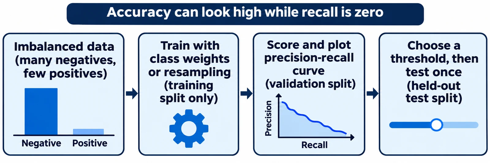
Some of the most useful machine learning problems involve rare events. Examples are fraudulent payments, equipment failures and uncommon diseases. In these problems, one outcome is far less common than the other, so a model can score well by almost never predicting the rare one.

This article explains how to train and evaluate a classifier when one outcome is uncommon. A classifier is a model that puts each example into a category, such as "fraud" or "not fraud". You will learn which metrics to trust, what class weights and resampling do, and how to pick a decision threshold. One illustrative example runs through the whole article.

Article index

• What class imbalance means
• Why accuracy misleads
• Precision, recall and average precision
• Class weights and resampling
• Choosing a decision threshold
• Privacy, fairness and security limits
• A worked example
• Common mistakes
• Recap
• Research Sources

What class imbalance means

A dataset is class-imbalanced when one label is considerably more common than the other. The common label is the majority class. The uncommon label is the minority class. Google's Machine Learning Crash Course says such datasets are far more common in the real world than balanced ones, and gives fraudulent card purchases (under 0.1% of transactions) and a rare virus (under 0.01% of patients) as examples. Source: Google Machine Learning Crash Course.

The same page separates mild from severe imbalance. With mild imbalance, training is usually fine because even small batches tend to contain both classes. With severe imbalance, the page says the data "might not contain enough minority class examples for proper training". It gives no numeric cutoff, so treat the labels as a rule of thumb.

The rare class is usually the one you care about. That mismatch between frequency and importance is the root of every problem in this article.

Why accuracy misleads

Accuracy is the share of predictions that are correct. If only 1 in 100 examples is positive, a model that always answers "negative" is 99% accurate. It is also useless, because it finds none of the cases you wanted. The Google course notes that accuracy is usually a poor metric for imbalanced datasets.

This is why you should look at the minority class directly. Two questions matter. Of the cases the model flagged, how many were real? Of the real cases, how many did the model find? Those two questions lead to precision and recall.

Precision, recall and average precision

Precision is the share of flagged cases that are truly positive. Recall is the share of truly positive cases that the model flagged. A model usually gives each example a score. Moving the cut-off score up raises precision and lowers recall, and moving it down does the reverse.

A precision-recall curve plots precision against recall across every possible cut-off. Average precision (AP) summarizes that curve in one number. The scikit-learn documentation defines AP as a weighted mean of precisions, where each weight is the increase in recall from the previous threshold. It also says this version is not interpolated, and that the trapezoidal-rule area under the curve "can be too optimistic". Source: scikit-learn average_precision_score (docs for version 1.9.1).

What about the more familiar ROC curve (receiver operating characteristic)? It plots the true positive rate against the false positive rate. Saito and Rehmsmeier, in a 2015 PLOS ONE paper, argue that ROC plots can be deceptive on imbalanced data. In their simulations, ROC curves stayed unchanged between balanced and imbalanced sets, and "only PRC changes with the ratio of positives and negatives". They strongly recommend precision-recall plots for imbalanced binary classification. Source: Saito and Rehmsmeier, PLOS ONE, 4 March 2015.

Here is my explanation of why. The false positive rate divides by all negatives. When negatives are huge, hundreds of false alarms still produce a tiny rate. Precision divides by flagged cases, so those false alarms show up directly. ROC is not wrong, but it can hide a problem that precision exposes.

Class weights and resampling

Training can pay more attention to the minority class in two broad ways. You can change how much each error costs, or you can change the training data itself.

Class weights

A class weight scales how much each example of a class contributes to the training loss, which is the number the model tries to reduce. In scikit-learn's LogisticRegression, class_weight accepts a dictionary such as {0: 1, 1: 5} or the string "balanced". The documentation says "balanced" sets weights inversely proportional to class frequencies using n_samples / (n_classes * np.bincount(y)). With 90 examples of class 0 and 10 of class 1, that gives about 0.56 and 5.0. Source: scikit-learn LogisticRegression.

Resampling

Resampling changes the training set. Random over-sampling copies minority examples, drawn with replacement. SMOTE (Synthetic Minority Oversampling Technique) instead creates new points. According to the imbalanced-learn documentation, it picks a minority sample, picks one of its nearest neighbors, and generates a point on the line between them. Source: imbalanced-learn over-sampling guide.

The same guide warns that SMOTE may connect inliers and outliers, which can lead to a suboptimal decision function. It also says SMOTENC is not designed for purely categorical data. Synthetic data is not free extra information. It is a guess about what the minority class looks like between known points.

A third option is to downsample the majority class and then upweight it. Google's course describes downsampling by a factor of 25, which turns a 99%/1% split into roughly 80%/20%. It then multiplies the majority-class loss by 25 to correct the prediction bias that downsampling adds. Both factors are hyperparameters, which are settings you tune by experiment. Source: Google Machine Learning Crash Course.

One rule applies to every method. Resample only the training data. The imbalanced-learn Pipeline documentation says its samplers "are only applied during fit", which keeps the evaluation data untouched. Source: imbalanced-learn Pipeline.

Choosing a decision threshold

A model outputs a score. A decision threshold turns that score into a yes or no. In binary classification, scikit-learn's predict returns the positive class when predict_proba is above 0.5, or when decision_function is above 0. The documentation calls these rules "not ideal for most use cases". It gives a tumor-detection case where a missed cancer costs more than an extra follow-up test, so a lower threshold may suit better. Source: scikit-learn, tuning the decision threshold.

The same page describes TunedThresholdClassifierCV, which picks the threshold by cross-validation to maximize a metric you choose. Its default metric is balanced accuracy, and the page advises picking a metric that fits your use case. It also warns that tuning on the data used for training risks overfitting, and that built-in scorers assume a default positive label. If your rare class is not the default, build a scorer with the right pos_label.

The threshold is a business and safety decision, not a purely technical one. Someone must decide how many false alarms are acceptable for each missed case.

Privacy, fairness and security limits

The rest of this section is my own explanation, not a documented finding from the sources above.

Privacy. Rare-class records are often the most sensitive, such as patients with a rare condition. Copying them many times with random over-sampling makes each one weigh more in training. SMOTE points are blends of real records, so do not assume they are anonymous. Keep resampled data under the same access controls as the original.

Fairness. A group that is small in your data may also have few positive cases. Overall precision and recall can look fine while a subgroup fares badly. Report the metrics per group when the model affects people.

Security. In fraud and abuse settings, attackers change behavior once they learn what gets flagged. A threshold tuned last quarter may not hold. Re-check the precision-recall curve on recent data on a schedule.

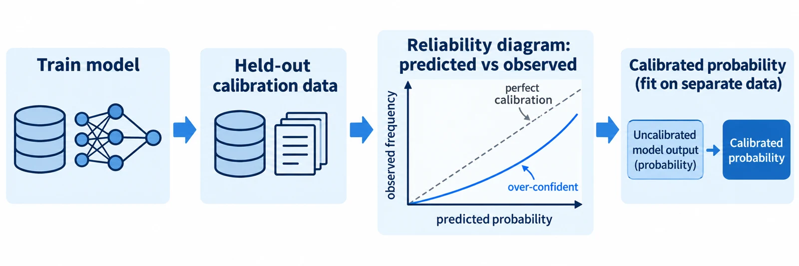
Probabilities. Weighting and resampling shift a model's scores away from real-world frequencies. Do not read a "0.8" from a reweighted model as an 80% chance. Recalibrate first if you need true probabilities.

A worked example

Illustrative scenario, not a test result. The numbers below are invented to show the arithmetic. Imagine a payment system with 10,000 transactions, of which 100 (1%) are fraud. The steps use the metrics defined above.

Prerequisites. Python with scikit-learn (the documentation I opened is for version 1.9.1, so check your installed version) and, for SMOTE, the imbalanced-learn package. You need labeled data with a clear positive class.

1. Set a baseline. Input: the 10,000 labels. A model that always says "not fraud" is right 9,900 times, so accuracy is 99%. Result: recall is 0%. Why it matters: any real model must beat this baseline on recall and precision, and accuracy cannot show that.
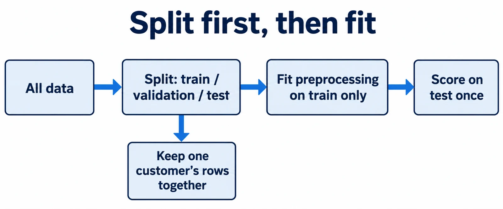
2. Split first. Input: the full dataset. Hold out a validation set and a test set before any resampling, and keep the fraud share similar in each split. This is called stratifying. Result: all three parts contain fraud cases. Why it matters: it keeps the evaluation honest.
3. Train with class weights. Input: the training split only. Fit a model with class_weight="balanced". Result: errors on fraud now count more in the loss. Why it matters: the model can no longer ignore the 1% class cheaply.
4. Score and read the table. Input: validation scores and a first threshold. Suppose the model flags 200 transactions: 60 are fraud (true positives) and 140 are not (false positives). So 40 frauds are missed and 9,760 legitimate transactions pass. Result: precision is 60/200 = 30%, recall is 60/100 = 60%, and accuracy is 9,820/10,000 = 98.2%. Why it matters: accuracy fell below the do-nothing baseline of 99%, yet the model is far more useful.
5. Compare with ROC. Input: the same counts. The false positive rate is 140/9,900, about 1.4%, so specificity is about 98.6%. Result: this looks excellent on a ROC plot while 7 in 10 alerts are false. Why it matters: it shows the gap Saito and Rehmsmeier describe.
6. Move the threshold. Input: a lower cut-off. Suppose the model now flags 400 transactions, with 75 fraud and 325 not fraud. Result: recall rises to 75%, and precision falls to 75/400 = 18.75%. Why it matters: a person must decide whether 15 more caught frauds justify 185 more false alarms for the review team.
7. Test once. Input: the chosen threshold and the untouched test split. Compute precision, recall and average precision a single time. Result: the numbers you report. Why it matters: choices made on the test set would make it another validation set.

A minimal sketch of steps 2 and 3 follows. It is example code, not output from a run, and it assumes you already have a feature table X and labels y with 1 as the rare class.

from sklearn.linear_model import LogisticRegression
from sklearn.metrics import average_precision_score
from sklearn.model_selection import train_test_split

X_train, X_test, y_train, y_test = train_test_split(
    X, y, test_size=0.2, stratify=y, random_state=0
)
model = LogisticRegression(class_weight="balanced", max_iter=1000)
model.fit(X_train, y_train)
scores = model.predict_proba(X_test)[:, 1]
print(average_precision_score(y_test, scores))

To check the result, confirm that y_test contains positives and that the printed value is a number between 0 and 1. If it fails with an error about a missing class, your split has no positives, so use a larger dataset or fewer splits. If AP is close to the positive share of the data, the model has learned little. Look at the features and labels before touching resampling.

Common mistakes

• Judging by accuracy. Report precision, recall and average precision for the rare class instead.
• Resampling before splitting. Copies or synthetic neighbors of one record can land in both training and test sets, which inflates scores. Split first, then resample inside the training fold, for example with the imbalanced-learn Pipeline.
• Keeping the 0.5 threshold by habit. Treat the threshold as a setting you choose on validation data.
• Tuning the threshold on training data. The scikit-learn page warns this risks overfitting. Use cross-validation or a separate validation set.
• Trusting reweighted probabilities. After weighting or resampling, scores no longer match real frequencies. Recalibrate if you must quote a probability.
• Using a ROC curve alone. Pair it with a precision-recall curve, and report the positive share so readers can judge the numbers.
• Applying SMOTE to categorical-only data. The imbalanced-learn guide says SMOTENC is not designed for it. Use SMOTEN for purely categorical features, or try class weights first.

Recap

• When one outcome is rare, accuracy can look excellent while the model finds nothing.
• Judge the rare class with precision, recall and average precision, and read a precision-recall curve alongside any ROC curve.
• Class weights and resampling make training pay attention to the minority class, but apply resampling only to training data.
• The decision threshold is a choice about the cost of false alarms versus misses. Tune it on validation data, then test once.
• Rare-class records raise privacy, fairness and adversarial concerns, so protect the data, report per-group results and recheck over time.

Research Sources

• Saito and Rehmsmeier, "The Precision-Recall Plot Is More Informative than the ROC Plot When Evaluating Binary Classifiers on Imbalanced Datasets", PLOS ONE, 2015
• scikit-learn documentation: average_precision_score
• scikit-learn documentation: LogisticRegression and class_weight
• scikit-learn documentation: tuning the decision threshold for class prediction
• imbalanced-learn documentation: over-sampling
• imbalanced-learn documentation: Pipeline
• Google Machine Learning Crash Course: Datasets, generalization, and overfitting — imbalanced datasets